


Time management is very much important in IIT JAM. The eduncle test series for IIT JAM Mathematical Statistics helped me a lot in this portion. I am very thankful to the test series I bought from eduncle.
Nilanjan Bhowmick AIR 3, CSIR NET (Earth Science)


Nisha Sharma posted an Question
September 15, 2021 • 22:37 pm
![]() 30 points
30 points
- UGC NET
- Commerce
Run total cost total cost (ltc) refers to the minimum cost at which given level of output can be produced. ac afasky, *the long run total cost of production is
Run Total Cost Total Cost (LTC) refers to the minimum cost at which given level of output can be produced. Ac afasky, *the long run total cost of production is the least possible cost of producing any given level 0 inputs are variable." LTC represents the least cost of different quantities of output. LTC is always to short run total cost, but it is never more than short run cost. STC LTC STC TC STC O Output Q Q Q Fig.:LTC Curve wn in Figure, short run total costs curves; STC, STC,, and STC, are shown depicting different C curve is made by joining the minimum points of short run total cost curves. Therefore, LTC en urves.
1 Answer(s)
Answer Now
- 0 Likes
- 3 Comments
- 0 Shares
-
Rucha rajesh shingvekar
![best-answer]()
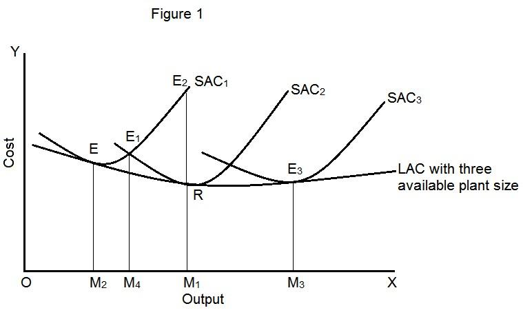
Long Run Cost Curves The long run is different from the short run in the variability of factor inputs. Accordingly, long-run cost curves are different from short-run cost curves. This lesson introduces you to Long run Total, Marginal and Average costs. You will learn the concepts, derivation of cost curves and graphical representation by way of diagrams and solved examples. The Concept of the Long Run The long run refers to that time period for a firm where it can vary all the factors of production. Thus, the long run consists of variable inputs only, and the concept of fixed inputs does not arise. The firm can increase the size of the plant in the long run. Thus, you can well imagine no difference between long-run variable cost and long-run total cost, since fixed costs do not exist in the long run. Long Run Total Costs Long run total cost refers to the minimum cost of production. It is the least cost of producing a given level of output. Thus, it can be less than or equal to the short run average costs at different levels of output but never greater. graphically deriving the LTC curve, the minimum points of the STC curves at different levels of output are joined. The locus of all these points gives us the LTC curve.Long Run Average Cost Curve Long run average cost (LAC) can be defined as the average of the LTC curve or the cost per unit of output in the long run. It can be calculated by the division of LTC by the quantity of output. Graphically, LAC can be derived from the Short run Average Cost (SAC) curves.While the SAC curves correspond to a particular plant since the plant is fixed in the short-run, the LAC curve depicts the scope for expansion of plant by minimizing cost.Derivation of the LAC Curve Note in the figure, that each SAC curve corresponds to a particular plant size. This size is fixed but what can vary is the variable input in the short-run. In the long run, the firm will select that plant size which can minimize costs for a given level of output.You can see that till the OM1 level of output it is logical for the firm to operate at the plat size represented by SAC2. If the firm operates at the cost represented by SAC2 when producing an output level OM2, the cost would be more.So in the long run, the firm will produce till OM1 on SAC2. However, till an output level represented by OM3, the firm can produce at SAC2, after which it is profitable to produce at SAC3 if the firm wishes to minimize costs.Thus, the choice, in the long run, is to produce at that plant size that can minimize costs. Graphically, this gives us a LAC curve that joins the minimum points of all possible SAC curves, as shown in the figure. Thus, the LAC curve is also called an envelope curve or planning curve. The curve first falls, reaches a minimum and then rises, giving it a U-shape.We can use returns to scale to explain the shape of the LAC curve. Returns to scale depict the change in output with respect to a change in inputs. During Increasing Returns to Scale (IRS), the output doubles by using less than double inputs. As a result, LTC increases less than the rise in output and LAC will fall.Constant Returns to Scale (CRS), the output doubles by doubling the inputs and the LTC increases proportionately with the rise in output. Thus, LAC remains constant. Decreasing Returns to Scale (DRS), the output doubles by using more than double the inputs so the LTC increases more than proportionately to the rise in output. Thus, LAC also rises. This gives LAC its U-shape.Long Run Marginal Cost Long run marginal cost is defined at the additional cost of producing an extra unit of the output in the long-run i.e. when all inputs are variable. The LMC curve is derived by the points of tangency between LAC and SAC. Note an important relation between LMC and SAC here. When LMC lies below LAC, LAC is falling, while when LMC is above LAC, LAC is rising. At the point where LMC = LAC, LAC is constant and minimum.
![cropped2993965622227370409.jpg]()
-
Nisha sharma
rucha mam please xplain me
Do You Want Better RANK in Your Exam?
Start Your Preparations with Eduncle’s FREE Study Material
- Updated Syllabus, Paper Pattern & Full Exam Details
- Sample Theory of Most Important Topic
- Model Test Paper with Detailed Solutions
- Last 5 Years Question Papers & Answers
Sign Up to Download FREE Study Material Worth Rs. 500/-


Priya sarda
The long run refers to that time period for a firm where it can vary all the factors of production. Thus, the long run consists of variable inputs only, and the concept of fixed inputs does not arise. The firm can increase the size of the plant in the long run. Thus, you can well imagine no difference between long-run variable cost and long-run total cost, since fixed costs do not exist in the long run. Long Run Total Costs Long run total cost refers to the minimum cost of production. It is the least cost of producing a given level of output. Thus, it can be less than or equal to the short run average costs at different levels of output but never greater. In graphically deriving the LTC curve, the minimum points of the STC curves at different levels of output are joined. The locus of all these points gives us the LTC curve.